Research compendium for Kohler, Brumbaugh, and Bocinsky (2025)
This R-based research compendium supports an analysis of climate variability and its impact on ancestral Pueblo demography in the Chaco Regional System. It draws on high-resolution paleoclimate reconstructions and spatial regional boundaries to estimate the frequency and duration of agricultural potential over time, and their relationship to the demography of the region.
When using the code included in this research compendium, please cite all of the following:
Kohler, Timothy A., Laura E. Brumbaugh, and R. Kyle Bocinsky. How Many People lived in the Chaco Regional System, and Why It Matters. KIVA, In review.
Kohler, Timothy A., Laura E. Brumbaugh, and R. Kyle Bocinsky. Research compendium for: How Many People lived in the Chaco Regional System, and Why It Matters, 2025. Version 1.0.0. Zenodo. [DOI]
Study Regions
The VEPIIN Study Area
The VEPIIN study area in the Central Mesa Verde region was somewhat arbitrarily defined to encompass the great Sage Plin, Mesa Verde National Park, and Canyons of the Ancients National Monument, as well as the expend of hte Dolores Archaeological Program in Southwestern Colorado. Was aligned to the NAD83 UTM zone 12N coordinate reference system, and sedigned such that even numbers 200m-by-200m might be included along each axis.
Code
## This creates a geojson of the VEPIIN study areaif(!file.exists("data-raw/vepiin.geojson"))c(xmin =672800, xmax =740000, ymin =4102000, ymax =4170000) %>% sf::st_bbox(crs =26912) %>% sf::st_as_sfc() %>% sf::st_transform("EPSG:4326") %>% sf::write_sf("data-raw/vepiin.geojson",delete_dsn =TRUE)
The Chaco Regional System
As described in the main paper, we develop boundaried for the spatial extent of the Chaco Regional System using a database of Chacoan outlier sites compiled by Van Dyke and colleagues (2016). We eliminated all site types other than great houses, and sorted the sites into temporal groups. We then categorized the sites as being included in one or several of our time periods: Early, Late, and Post-Chaco. Sites are included in more than one of these groups if their occupations spanned the temporal cut-offs.
The Early Chaco group contains 60 sites with occupation at any point between 850-1039, including sites whose occupations continue after 1039, so long as the initial occupation occurred prior to 1039. (All dates herein are AD/CE).
The Late Chaco group contains 168 sites with occupation between 1040 and 1149, including sites whose occupations began before and/or continued after these dates.
The Post-Chaco group contains 107 sites with occupation from 1150 to 1300; this includes great houses that were constructed during the two earlier CRS periods as well as great houses with initial construction between 1150 and 1300.
Brumbaugh developed a method, detailed in the main paper, to generate a reasonable boundary for the Chaco Regional System during each period. Briefly, we removed border sites that lacked definitive Chacoan architectural attributes, then used ArcGIS Pro to buffer each site by one kilometerand define a concave hull of threshold 0.7 around the sites.
Code
chaco_regions <-list(`E CRS (850–1040)`="data-raw/EarlyChacoRegion_LatLong.geojson",`L CRS (1040–1150)`="data-raw/LateChacoRegion_LatLong.geojson",`P CRS (1150–1300)`="data-raw/PostChacoRegion_LatLong.geojson",`VEPIIN (850–1300)`="data-raw/vepiin.geojson" ) %>% purrr::map_dfr(sf::read_sf, .id ="region") %>% dplyr::select(region) %>% sf::st_transform("EPSG:4269") %>% sf::st_cast("MULTIPOLYGON")chaco_region_colors <-c(paletteer::paletteer_c("scico::batlow", n =4)[1:3],"black") %>% magrittr::set_names(c("E CRS (850–1040)","L CRS (1040–1150)","P CRS (1150–1300)","VEPIIN (850–1300)" ))# Show a table of region areas calculated in NAD83, Zone 12 units (as reported in the paper)chaco_regions %>% sf::st_transform(26912) %>% dplyr::mutate(Region = region,Area = sf::st_area(geometry) %>% units::set_units("km^2") %>%round()) %>% sf::st_drop_geometry() %>% dplyr::select(Region, Area)
Figure 1: Extent of the Chaco Regional System during the Early CRS (AD 850-1039), Late CRS (1040-1149), and Post-CRS (1150-1300), with the VEPIIN area. Extrema identified for the Early and Late CRS. This map in the main manuscript was made in QGIS by Laura Brumbaugh.
Code
# Get state boundaries from the US Census for mappingstates <- tigris::states(cb =TRUE,progress_bar =FALSE) %>% dplyr::filter(NAME %in%c("Colorado","Utah","New Mexico","Arizona"))#> Retrieving data for the year 2024# Define a plotting area around the "Chaco Basin"chaco_basin <- sf::st_bbox(c(xmin =-110.35,xmax =-106.9, ymin =34.1,ymax =37.8), crs ="EPSG:4269") %>% sf::st_as_sfc() %>% sf::st_bbox()# Create a faceting dataset that always includes VEPIINchaco_regions_facet <- chaco_regions %>% dplyr::rename(lyr = region) %>% { dplyr::bind_rows(., dplyr::filter(., lyr =="VEPIIN (850–1300)") %>%# THIS PIPE TYPE MATTERS tidyr::uncount(3) |> dplyr::mutate(lyr = dplyr::filter(., lyr !="VEPIIN (850–1300)")$lyr)) } %>% dplyr::filter(lyr !="VEPIIN (850–1300)")# A function that makes a handsome faceted plotplot_map_array <-function(x, filename, limits, name,facet =TRUE, ...){ out <- (ggplot() +geom_spatraster(data = x,na.rm =TRUE) +facet_wrap(~lyr) + paletteer::scale_fill_paletteer_binned("scico::batlow",# dynamic = TRUE,na.value ="transparent",n.breaks =10,show.limits =TRUE,limits = limits,name = name, ...) +geom_sf(data = states,fill =NA, color ="white") + {if(facet)geom_sf(data = chaco_regions_facet,fill =NA,color ="white") } +theme_void() +theme(legend.position ="left",legend.justification =0.5,legend.title =element_text(angle =90, hjust =0.5),legend.title.position ="left",legend.key.height =unit(0.15, "npc")) +coord_sf(crs ="EPSG:4269",xlim = chaco_basin[c("xmin", "xmax")],ylim = chaco_basin[c("ymin", "ymax")],expand =TRUE ) )return(out) }
Dryland Maize Farming Niche
Here, we derive a dryland maize farming niche from paleoclimate reconstructions provided by the Synthesizing Knowledge of Past Environments (SKOPE) project. This code computes the Maize Farming Niche (MFN) for the U.S. Southwest by combining gridded paleoclimate reconstructions of precipitation and growing degree days (GDD), which we download from Amazon S3. We begin by defining output file paths and retrieving the relevant PaleoCAR raster data. We then generate a binary raster indicating areas suitable for maize cultivation—those where both precipitation and GDD exceed specified thresholds (e.g., GDD > 1000). If this MFN raster does not already exist, we compute it and save it to disk. Next, we extract mean and standard deviation MFN values for each region in chaco_regions, summarizing the results in an Excel spreadsheet. Finally, we compute average MFN conditions for key archaeological periods (Early, Late, Post-Chaco, and VEPIIN) by averaging the relevant yearly layers in the raster stack.
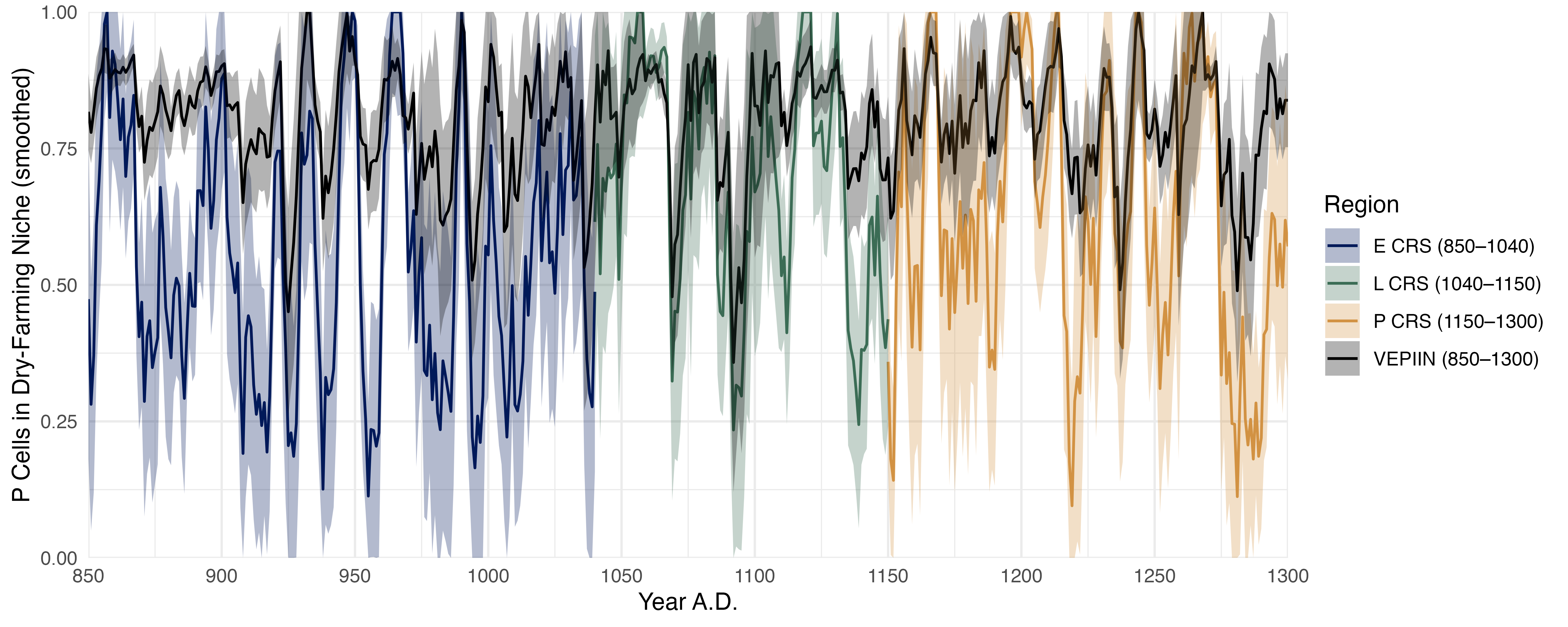
Figure 2: Average proportion of cells within the maize dry-farming niche through time for the four regions outlined in Figure 1. E CRS (etc.) indicates Early Chaco Regional System. The proportion of cells in the dry-farming niche is determined by tree-ring-based estimates of temperature and precipitation (Bocinsky and Kohler 2014). Cells with precipitation >= 250mm and Growing Degree Days >= 1000 are deemed within the niche. The point estimate plotted for each year is based on a linear regression of year on maize-niche proportion, using a moving window containing the previous 10 years. For example, the value plotted for AD 900 is the linear prediction using niche proportions from AD 890 to 899. The standard error for each regression is used to calculate 80% CIs around the point estimates, shown by the shaded areas. A simpler view of these data, by decadal means, is presented in Figure S1.
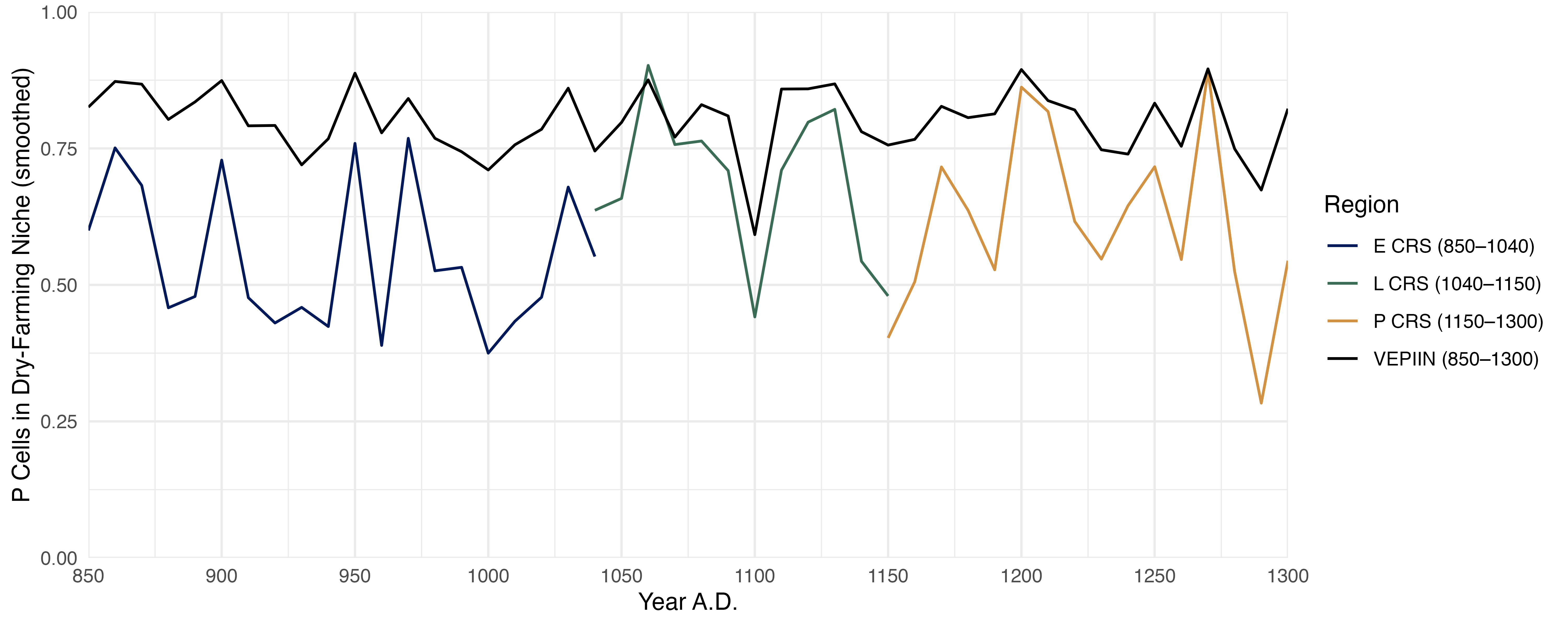
In Figure S1, we present a simplified version of Figure 2 using decadal means, as calculated here.
Figure S1: Average proportion of cells within the maize dry-farming niche by decade for the four regions outlined in Figure 1. The proportion of cells in the dry-farming niche is determined by tree-ring-based estimates of temperature and precipitation (Bocinsky and Kohler 2014). Cells with precipitation >= 300mm and Growing Degree Days >= 1000 are deemed within the niche. Each vertex represents the mean proportion of the study area within the maize niche for the preceding 10 years (i.e., the vertex at 860 represents the years 850-859). This represents the most temporally relevant knowledge a Pueblo farmer in that year would have about recent agricultural conditions.This is a simplified view of the more detailed maize niche data presented in the main paper, Figure 2.
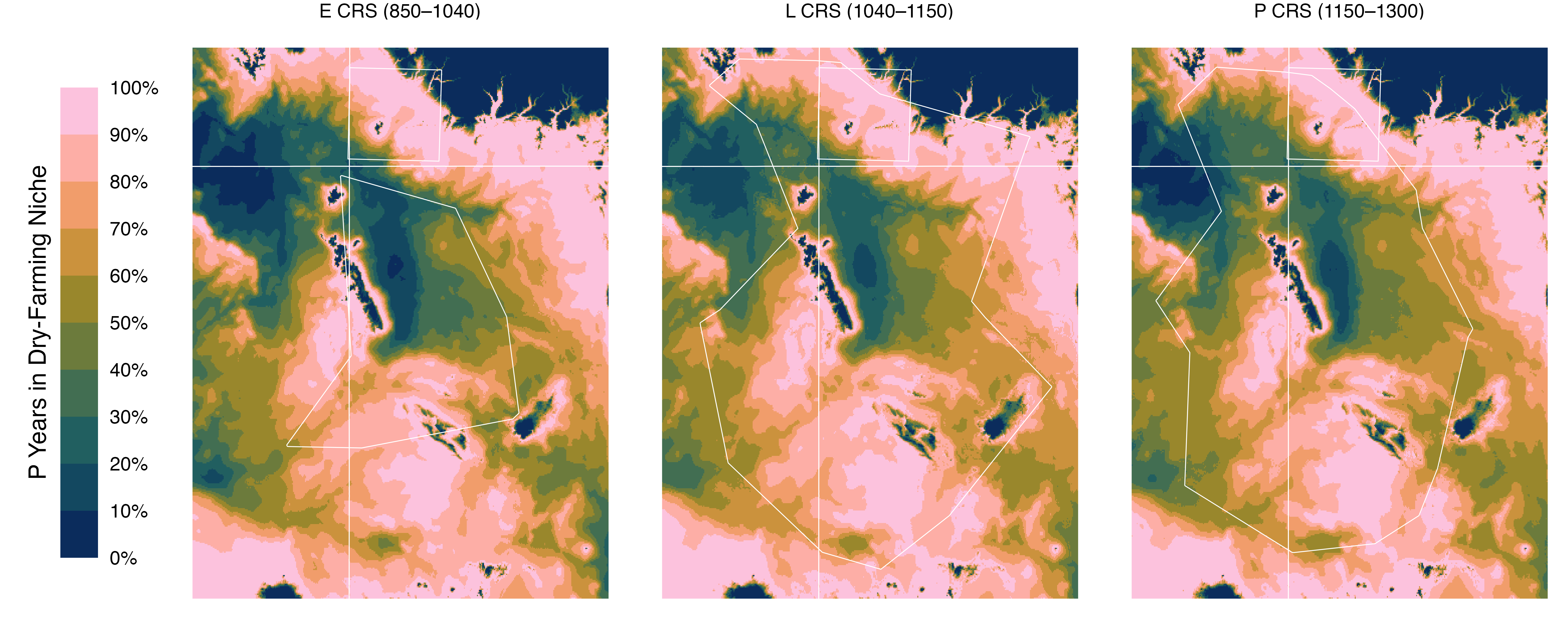
The Maize Farming Niche may be visualized as the proportion of years within a given period that meet the niche thresholds (here, 250 mm of water year precipitation and 1000 growing degree days).
Figure S2: Percent of years in the maize dry-farming niche across Chacoan regions during key cultural periods.
Pre-European Net Primary Productivity
To model pre-European Net Primary Productivity (NPP), we estimated potential landscape productivity in the absence of modern irrigation and disturbance, establishing a baseline for past agricultural suitability. We used MODIS 250m annual NPP data for the years 2002, 2007, 2012, and 2017 (Rollins 2009), along with MIRAD irrigated lands data (Pervez and Brown 2010), Landfire datasets (Biophysical Settings, Existing Vegetation Types, Historical Disturbance; (Nelson et al. 2013; Rollins 2009), and PRISM 800m elevation data. We reprojected and aligned all datasets to a common spatial template based on the 800m PRISM dataset. For model training, we retained irrigated and disturbed pixels, but we excluded them during prediction to simulate pre-European conditions.
This section of the code prepares the environmental raster datasets at a common resolution and extent. Specifically, we resample, reclassify, and align data on productivity, irrigation, vegetation, disturbance, and elevation to a shared spatial template.
Data preparation
1. Establish a Template Raster
We create a single-layer raster template based on the Maize Farming Niche data to use as a consistent spatial reference for projection and alignment.
We extract the annualNPP layer, project it to the template grid using bilinear interpolation, and save the output as a compressed raster stack.
3. Irrigated Lands (MIRAD)
We query and download MIRAD-derived irrigated lands data from the USGS ScienceBase repository (DOI:10.5066/P9NA3EO8).
We load the relevant 250m rasters, project them to our template using max resampling (preserving irrigated presence), and save the result as a binary raster.
We unzip the file, extract the raster and its corresponding classification CSV.
We project it to our template using mode resampling (preserving dominant class).
We recategorize factor levels to consolidate similar vegetation types or correct naming inconsistencies.
We then assemble the BPS, EVT, and HDist layers into a single multi-layer raster object.
5. PRISM Elevation
We download the 800-meter DEM from the PRISM Climate Group via a virtual file system call (/vsicurl).
We crop it to the template extent and save the result for elevation analysis.
Code
template <- terra::rast(niche_periods) %>% terra::rast(nlyr =1)## MODIS NPP (250m)if(!file.exists("data-derived/modis_npp_swus_paleocar.tif")){ get_npp <-function(years =c(2002, 2007, 2012, 2017)){ modis_npp_urls <-paste0("http://files.ntsg.umt.edu/data/NTSG_Products/MOD17/MODIS_250/modis-250-npp/modis-250-npp-",years,".tif") destfiles <-file.path("data-raw",basename(modis_npp_urls))download_files(urls = modis_npp_urls,destfiles = destfiles ) %$% destfile %>% purrr::map(terra::rast) %>% purrr::map(\(x) x$annualNPP) %>% terra::rast() %>% magrittr::set_names(paste0(years, " 250m MODIS NPP")) } modis_npp <-get_npp() %>% terra::project(template,method ="bilinear",filename ="data-derived/modis_npp_swus_paleocar.tif",datatype ="INT2U",overwrite =TRUE,gdal =c("COMPRESS=ZSTD"),memfrac =0.9)}modis_npp <- terra::rast("data-derived/modis_npp_swus_paleocar.tif")## Irrigated Landsif(!file.exists("data-derived/mirad_irrlands_swus_paleocar.tif")){ get_scibase <-function(uri, filename){ file <- stringr::str_replace(filename, ".zip", ".tif") %>% stringr::str_replace("m_","_")if(!file.exists(filename)) { uri %>%download.file(destfile =file.path("data-raw", filename)) }file.path("/vsizip", "data-raw", filename, stringr::str_remove(filename, ".zip"), file) %>% terra::rast() } mirad_irrlands <-query_sb_doi("10.5066/P9NA3EO8") %>% purrr::pluck(1, "files") %>% purrr::map(\(x)x[c("title", "name", "downloadUri")]) %>% purrr::list_transpose(simplify =TRUE) %>% tibble::as_tibble() %>% dplyr::filter(stringr::str_detect(title, "250m"), stringr::str_detect(title, "All", negate =TRUE)) %>% dplyr::rowwise() %>% dplyr::mutate(rast =list(get_scibase(uri = downloadUri,filename = name ) )) %$% {magrittr::set_names(rast, title)} %>% terra::rast() %>% terra::project(template,method ="max",filename ="data-derived/mirad_irrlands_swus_paleocar.tif",datatype ="INT1U",overwrite =TRUE,gdal =c("COMPRESS=ZSTD", "NBITS=1"),memfrac =0.9)}mirad_irrlands <- terra::rast("data-derived/mirad_irrlands_swus_paleocar.tif")# Landfire BPS, Historical Disturbance, and Existing Vegetation Typesif(c(bps ="data-derived/landfire_bps_swus_paleocar.tif",disturbance ="data-derived/landfire_disturbance_swus_paleocar.tif",evt ="data-derived/landfire_evt_swus_paleocar.tif") %>%file.exists() %>%all() %>%not()){ read_and_write_landfire <-function(raster, levels, outfile){if(!file.exists(outfile)){ out <- terra::rast(raster) %>%`levels<-`( sf::read_sf(levels) %>% readr::type_convert() ) %>% terra::project( template,method ="mode",filename = outfile,datatype ="INT4U",overwrite =TRUE,gdal =c("COMPRESS=ZSTD"),memfrac =0.9 ) }return(outfile) } landfire <-c(bps ="https://www.landfire.gov/data-downloads/US_220/LF2020_BPS_220_CONUS.zip",disturbance ="https://www.landfire.gov/data-downloads/US_Disturbance/LF2023_HDist_240_CONUS.zip",evt ="https://www.landfire.gov/data-downloads/US_240/LF2023_EVT_240_CONUS.zip" ) %>% { tibble::tibble(dataset =names(.),downloads = . ) } %>% dplyr::mutate(destfiles =file.path("data-raw", basename(downloads)),destfiles =download_files(urls = downloads,destfiles = destfiles )$destfile ) %>% dplyr::mutate(rastfile = dplyr::case_match( dataset,"bps"~basename(destfiles) %>% stringr::str_replace("_CONUS.zip", ".tif") %>% stringr::str_replace("LF2020", "LC20"),"disturbance"~basename(destfiles) %>% stringr::str_replace("_CONUS.zip", ".tif") %>% stringr::str_replace("LF20", "LC") %>% stringr::str_replace("HDist", "HDst"),"evt"~basename(destfiles) %>% stringr::str_replace("_CONUS.zip", ".tif") %>% stringr::str_replace("LF20", "LC") ) %>%file.path("/vsizip", destfiles, stringr::str_remove(basename(destfiles), ".zip"),"Tif", .),levelsfile = dplyr::case_match( dataset,"bps"~ rastfile %>% stringr::str_replace("Tif", "CSV_Data") %>% stringr::str_replace(".tif", ".csv") %>% stringr::str_replace("LC20", "LF20"),"disturbance"~ rastfile %>% stringr::str_replace("Tif", "CSV_Data") %>% stringr::str_replace(".tif", ".csv") %>% stringr::str_replace("LC23", "LF23"),"evt"~ rastfile %>% stringr::str_replace("Tif", "CSV_Data") %>% stringr::str_replace(".tif", ".csv") %>% stringr::str_replace("LC23", "LF23") ) ) %>% dplyr::rowwise() %>% dplyr::mutate(rast =read_and_write_landfire(raster = rastfile,levels = levelsfile,outfile =file.path("data-derived", paste0("landfire_", dataset, "_swus_paleocar.tif"))) ) %>% dplyr::ungroup()}read_and_recat <-function(x, variable){ terra::rast(x) %>% terra::`activeCat<-`(variable) %>%as.data.frame(na.rm=FALSE) %>% tibble::as_tibble() %>% terra::setValues(template, values = .) %>% magrittr::set_names( x %>% basename %>% tools::file_path_sans_ext() ) }landfire <-list(bps =read_and_recat("data-derived/landfire_bps_swus_paleocar.tif",variable ="BPS_NAME"),evt =read_and_recat("data-derived/landfire_evt_swus_paleocar.tif",variable ="EVT_NAME"),disturbance =read_and_recat("data-derived/landfire_disturbance_swus_paleocar.tif",variable ="DIST_TYPE") ) %>% terra::rast()# Recode missing categorieslandfire$bps %<>%as.data.frame(na.rm=FALSE) %>% tibble::as_tibble() %>% dplyr::mutate(bps = forcats::fct_recode( bps,`Apacherian-Chihuahuan Semi-Desert Shrub-Steppe`="Apacherian-Chihuahuan Semi-Desert Grassland and Steppe",`Apacherian-Chihuahuan Semi-Desert Grassland`="Apacherian-Chihuahuan Mesquite Upland Scrub",`Chihuahuan Mixed Desert and Thornscrub`="Chihuahuan Mixed Desert and Thorn Scrub",`Chihuahuan Mixed Desert and Thornscrub`="Chihuahuan Mixed Desert and Thorn Scrub-Shrubland",`Chihuahuan Mixed Desert and Thornscrub`="Chihuahuan Mixed Desert and Thorn Scrub-Steppe",`Chihuahuan-Sonoran Desert Bottomland and Swale Grassland`="Chihuahuan-Sonoran Desert Bottomland and Swale Grassland-Alkali Sacaton",`Chihuahuan-Sonoran Desert Bottomland and Swale Grassland`="Chihuahuan-Sonoran Desert Bottomland and Swale Grassland-Tobosa Grassland",`Inter-Mountain Basins Aspen-Mixed Conifer Forest and Woodland`="Inter-Mountain Basins Aspen-Mixed Conifer Forest and Woodland-High Elevation",`Inter-Mountain Basins Aspen-Mixed Conifer Forest and Woodland`="Inter-Mountain Basins Aspen-Mixed Conifer Forest and Woodland-Low Elevation",`Inter-Mountain Basins Big Sagebrush Shrubland`="Inter-Mountain Basins Big Sagebrush Shrubland-Basin Big Sagebrush",`Inter-Mountain Basins Big Sagebrush Shrubland`="Inter-Mountain Basins Big Sagebrush Shrubland-Semi-Desert",`Inter-Mountain Basins Big Sagebrush Shrubland`="Inter-Mountain Basins Big Sagebrush Shrubland-Upland",`Inter-Mountain Basins Big Sagebrush Shrubland`="Inter-Mountain Basins Big Sagebrush Shrubland-Wyoming Big Sagebrush",`Inter-Mountain Basins Montane Sagebrush Steppe`="Inter-Mountain Basins Montane Sagebrush Steppe-Low Sagebrush",`Inter-Mountain Basins Montane Sagebrush Steppe`="Inter-Mountain Basins Montane Sagebrush Steppe-Mountain Big Sagebrush",`Rocky Mountain Gambel Oak-Mixed Montane Shrubland`="Rocky Mountain Gambel Oak-Mixed Montane Shrubland -Continuous",`Rocky Mountain Gambel Oak-Mixed Montane Shrubland`="Rocky Mountain Gambel Oak-Mixed Montane Shrubland-Patchy",`Rocky Mountain Lower Montane-Foothill Shrubland`="Rocky Mountain Lower Montane-Foothill Shrubland-No True Mountain Mahogany",`Rocky Mountain Lower Montane-Foothill Shrubland`="Rocky Mountain Lower Montane-Foothill Shrubland-True Mountain Mahogany",`Southern Rocky Mountain Ponderosa Pine Savanna`="Southern Rocky Mountain Ponderosa Pine Savanna-North",`Southern Rocky Mountain Ponderosa Pine Woodland`="Southern Rocky Mountain Ponderosa Pine Woodland-North",`Southern Rocky Mountain Ponderosa Pine Woodland`="Southern Rocky Mountain Ponderosa Pine Woodland-South",`Western Great Plains Closed Depression Wetland`="Western Great Plains Depressional Wetland Systems",`Western Great Plains Closed Depression Wetland`="Western Great Plains Depressional Wetland Systems-Playa",`Western Great Plains Closed Depression Wetland`="Western Great Plains Depressional Wetland Systems-Saline",`Western Great Plains Tallgrass Prairie`="Central Tallgrass Prairie",`Inter-Mountain Basins Wash`="Inter-Mountain Basins Montane Riparian Systems",`North American Warm Desert Riparian Systems`="North American Warm Desert Riparian Systems-Stringers",`North American Glacier and Ice Field`="Perennial Ice/Snow",`Northwestern Great Plains-Black Hills Ponderosa Pine Woodland and Savanna`="Northwestern Great Plains-Black Hills Ponderosa Pine Woodland and Savanna-Savanna",`Western Great Plains Badlands`="Western Great Plains Sparsely Vegetated Systems",`North American Warm Desert Badland`="North American Warm Desert Sparsely Vegetated Systems",`Rocky Mountain Alpine-Montane Wet Meadow`="Northern Rocky Mountain Conifer Swamp",`Barren-Rock/Sand/Clay`="Inter-Mountain Basins Sparsely Vegetated Systems",`Barren-Rock/Sand/Clay`="Rocky Mountain Alpine/Montane Sparsely Vegetated Systems",`Barren-Rock/Sand/Clay`="Inter-Mountain Basins Sparsely Vegetated Systems",`Northwestern Great Plains Floodplain Herbaceous`="Northwestern Great Plains Canyon",`Southern Rocky Mountain Ponderosa Pine Woodland`="Northwestern Great Plains Highland White Spruce Woodland",`Rocky Mountain Lodgepole Pine Forest`="Rocky Mountain Poor-Site Lodgepole Pine Forest",`Central Mixedgrass Prairie`="Western Great Plains Wooded Draw and Ravine",`Inter-Mountain Basins Big Sagebrush Steppe`="Inter-Mountain Basins Big Sagebrush Shrubland" ) ) %>% terra::setValues(template, values = .)landfire$evt %<>%as.data.frame(na.rm=FALSE) %>% tibble::as_tibble() %>% dplyr::mutate(evt = forcats::fct_recode( evt,`Central Mixedgrass Prairie`="Central Mixedgrass Prairie Grassland",`Central Mixedgrass Prairie`="Central Mixedgrass Prairie Shrubland",`Inter-Mountain Basins Curl-leaf Mountain Mahogany Woodland and Shrubland`="Inter-Mountain Basins Curl-leaf Mountain Mahogany Shrubland",`Inter-Mountain Basins Curl-leaf Mountain Mahogany Woodland and Shrubland`="Inter-Mountain Basins Curl-leaf Mountain Mahogany Woodland",`Rocky Mountain Subalpine/Upper Montane Riparian Systems`="Rocky Mountain Subalpine-Montane Riparian Shrubland",`Rocky Mountain Subalpine/Upper Montane Riparian Systems`="Rocky Mountain Subalpine-Montane Riparian Woodland", `Western Great Plains Floodplain Systems`="Western Great Plains Floodplain Herbaceous",`Western Great Plains Floodplain Systems`="Western Great Plains Floodplain Shrubland",`Western Great Plains Mesquite Woodland and Shrubland`="Western Great Plains Mesquite Shrubland",`North American Warm Desert Riparian Systems`="North American Warm Desert Riparian Woodland",`North American Warm Desert Riparian Systems`="North American Warm Desert Riparian Shrubland",`Rocky Mountain Montane Riparian Systems`="Rocky Mountain Lower Montane-Foothill Riparian Shrubland",`Rocky Mountain Montane Riparian Systems`="Rocky Mountain Lower Montane-Foothill Riparian Woodland",`Rocky Mountain Alpine/Montane Sparsely Vegetated Systems`="Rocky Mountain Alpine Bedrock and Scree",`Barren-Rock/Sand/Clay`="Colorado Plateau Mixed Bedrock Canyon and Tableland",`Barren-Rock/Sand/Clay`="Inter-Mountain Basins Shale Badland",`Barren-Rock/Sand/Clay`="Inter-Mountain Basins Playa",`Barren-Rock/Sand/Clay`="Inter-Mountain Basins Active and Stabilized Dune",`Barren-Rock/Sand/Clay`="Inter-Mountain Basins Volcanic Rock and Cinder Land",`Barren-Rock/Sand/Clay`="Rocky Mountain Cliff Canyon and Massive Bedrock",`Apacherian-Chihuahuan Semi-Desert Shrub-Steppe`="Edwards Plateau Limestone Shrubland",`Inter-Mountain Basins Big Sagebrush Steppe`="Inter-Mountain Basins Big Sagebrush Shrubland",`Inter-Mountain Basins Big Sagebrush Steppe`="Columbia Plateau Steppe and Grassland",`Inter-Mountain Basins Mixed Salt Desert Scrub`="Great Basin & Intermountain Ruderal Shrubland",`Barren-Rock/Sand/Clay`="Rocky Mountain Alpine/Montane Sparsely Vegetated Systems",`Barren-Rock/Sand/Clay`="North American Warm Desert Active and Stabilized Dune",`Apacherian-Chihuahuan Semi-Desert Shrub-Steppe`="North American Warm Desert Ruderal & Planted Scrub",`Barren-Rock/Sand/Clay`="North American Warm Desert Playa",`Inter-Mountain Basins Big Sagebrush Steppe`="Inter-Mountain Basins Cliff and Canyon",`Mojave Mid-Elevation Mixed Desert Scrub`="North American Warm Desert Bedrock Cliff and Outcrop",`North American Warm Desert Badland`="North American Warm Desert Pavement",`Inter-Mountain Basins Greasewood Flat`="Interior Western North American Temperate Ruderal Shrubland" ) ) %>% terra::setValues(template, values = .)#> Warning: There was 1 warning in `dplyr::mutate()`.#> ℹ In argument: `evt = forcats::fct_recode(...)`.#> Caused by warning:#> ! Unknown levels in `f`: Rocky Mountain Alpine/Montane Sparsely Vegetated Systems# PRISM Elevationif(!file.exists("data-derived/elev_swus_paleocar.tif")){ elev <- terra::rast("/vsizip//vsicurl/https://data.prism.oregonstate.edu/normals_bil/monthly/800m/dem/PRISM_us_dem_800m_bil.zip/PRISM_us_dem_800m_bil.bil") %>% terra::crop(template) %>% magrittr::set_names("elev") %>% terra::writeRaster(filename ="data-derived/elev_swus_paleocar.tif",datatype ="INT4S",overwrite =TRUE,gdal =c("COMPRESS=ZSTD"),memfrac =0.9 )}elev <- terra::rast("data-derived/elev_swus_paleocar.tif")
We trained LightGBM (Ke et al. 2017) quantile regression models to predict log-transformed NPP at the 10th, 50th, and 90th percentiles. Our models treated EVT, disturbance type, and irrigated lands as categorical predictors and elevation, latitude, and longitude as continuous predictors. After training, we used these models to generate NPP predictions across the study area under a no-irrigation, no-disturbance scenario. We visualized the resulting median (50%) NPP map as a baseline productivity surface (Figure S3). We then multiplied this surface by the proportion of years meeting Maize Farming Niche (MFN) thresholds to generate maps of “niche-attenuated NPP” (Figure S4). Finally, we normalized these values relative to the central Mesa Verde region to estimate relative productivity maps (Figure S5) that highlight agricultural potential across the Chaco Basin.
Estimating Pre-European Net Primary Productivity (NPP) Using Gradient Boosted Models
This code fits a quantile-based LightGBM (Gradient Boosted Machine) model to estimate pre-European NPP based on landscape characteristics in the U.S. Southwest. The process includes the following steps:
Data Assembly
We construct a spatial dataset (landscape_data) by combining:
LANDFIRE Biophysical Settings (BPS), Existing Vegetation Types (EVT), and Disturbance data
PRISM elevation
MODIS-derived NPP (for years 2002, 2007, 2012, 2017)
MIRAD irrigated lands
Data are merged by year and converted to tidy, long format.
Training Data Preparation
We convert categorical predictors to integers, remove missing values, and drop unused fields (e.g., year, BPS).
The response variable is the natural log of NPP plus one (log1p(NPP)), which helps handle skewed data.
Model Fitting
We fit three LightGBM quantile regression models, targeting the 10th, 50th, and 90th percentiles of NPP.
Models are trained using furrr::future_map() in parallel (multisession) to speed up computation.
Prediction
We simulate a “pre-European” landscape by assuming:
No irrigation (mirad_irrlands = 0)
No recent disturbance (disturbance = 'Non Disturbed')
We generate predictions for each quantile, back-transform the output with expm1(), and mask predictions to valid elevation areas.
Output
Predicted rasters are stacked and written to disk as "data-derived/pre-european_npp_swus.tif".
Load Results
The final raster stack is loaded into the object modeled_production for use in subsequent analysis.
This approach provides a modeled baseline for potential productivity in the absence of modern anthropogenic influences.
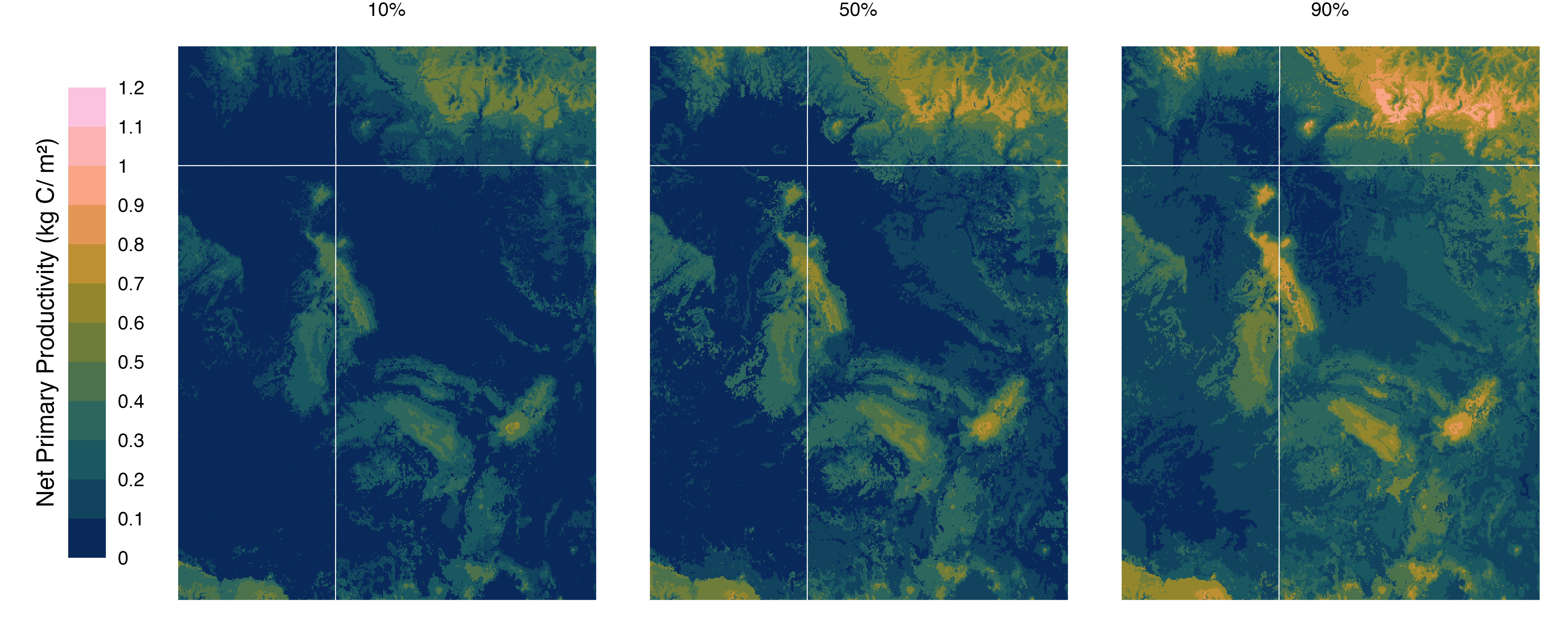
Figure S3: Estimated pre-European Net Primary Productivity (NPP) across the U.S. Southwest. We used LightGBM quantile regression to model 10th, 50th (median), and 90th percentile NPP under pre-European conditions—excluding modern irrigation and recent disturbances—based on MODIS NPP data, elevation, and land cover characteristics. The resulting maps provide a baseline of landscape productivity in kg C/m².
Calculating Relative Maize Productivity by Region
This code estimates relative maize productivity by archaeological region and period, scaling modeled productivity values by the mean within a reference region (VEPIIN, 850–1300 CE). This enables cross-regional comparison of potential maize farming success.
Define a Scaling Function
calculate_relative_raster() divides each cell in a raster (or raster stack) by the mean value within a given area of interest (AOI), so that the AOI’s mean becomes 1.
This normalizes productivity values relative to a baseline region.
Estimate Period-Specific Productivity
We multiply the maize niche mask for each period (niche_periods) by the median modeled pre-European NPP (modeled_production$"50%") to calculate potential maize productivity for each period.
Normalize to VEPIIN
We apply the scaling function to the productivity rasters using VEPIIN (850–1300 CE) as the reference AOI.
This produces relative_production, a raster stack where all values are scaled so that VEPIIN’s mean is 1.
Summarize by Region
For each region in chaco_regions, we extract the mean relative productivity.
The result is a region-wise summary table with scaled productivity values for each period.
Export Output
The final table, relative_production_regions, is written to CSV as data-derived/relative_productivity_<PPT_THRESHOLD>.csv.
This analysis helps contextualize agricultural potential across different regions by expressing it relative to a well-studied reference area.
Code
## A function that scales a raster proportional to the mean of an AOI. ## The mean of the AOI will be 1.calculate_relative_raster <-function(x, aoi){ x %>% terra::extract( aoi,fun = mean,na.rm =TRUE,touches =TRUE,ID =FALSE) %>% purrr::map2(.y =as.list(x), \(aoi, rast){ (rast / aoi) } ) %>% terra::rast() }niche_npp_periods <- niche_periods * modeled_production$`50%`relative_production <- niche_npp_periods %>%calculate_relative_raster(aoi = chaco_regions %>% dplyr::filter(region =="VEPIIN (850–1300)"))relative_production_regions <- chaco_regions %>% dplyr::left_join( relative_production %>% { tibble::tibble(region =names(.),relative_productivity = terra::as.list(.) ) } ) %>% dplyr::rowwise() %>% dplyr::mutate(relative_productivity = terra::extract( relative_productivity, sf::st_as_sf(geometry),fun = mean,na.rm =TRUE,touches =TRUE,ID =FALSE) %>%unlist() ) %>% dplyr::ungroup() %>% sf::st_drop_geometry() %T>% readr::write_excel_csv(paste0("data-derived/relative_productivity_", ppt_threshold, ".csv"))#> Joining with `by = join_by(region)`
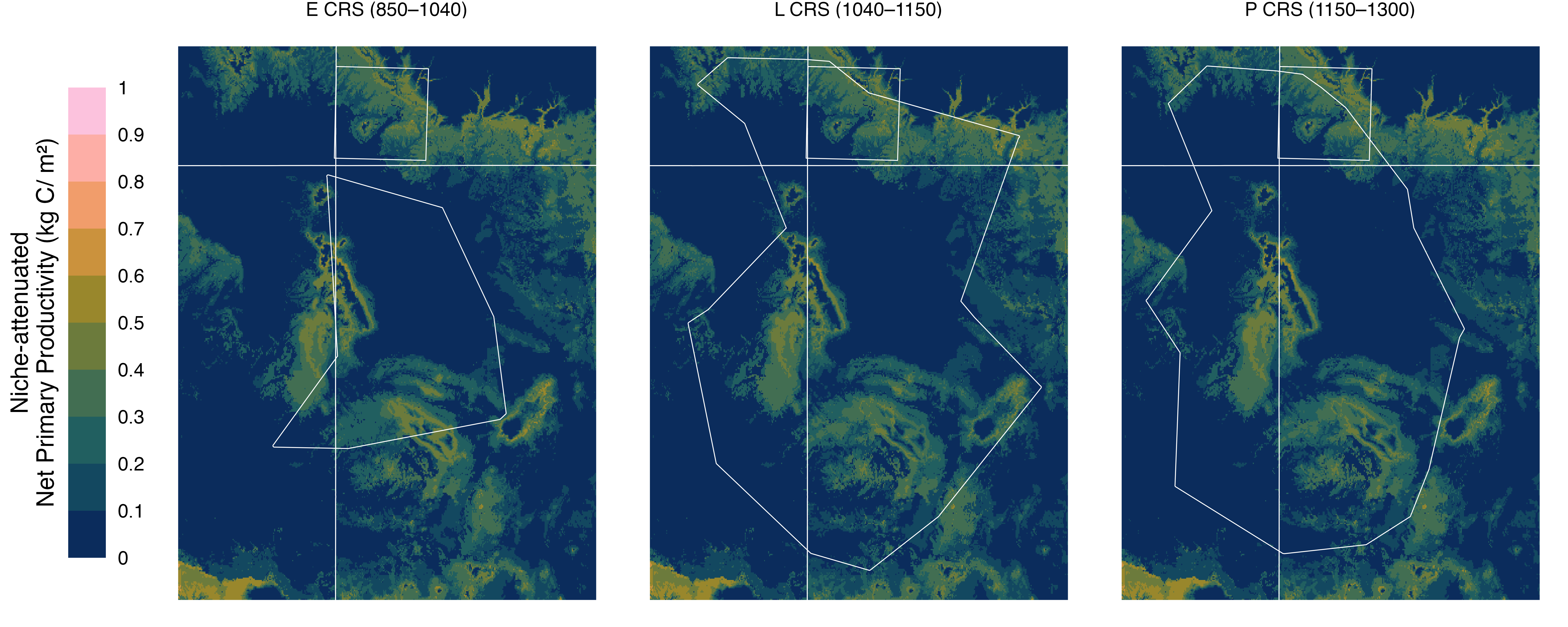
Figure S4: Niche-attenuated Net Primary Productivity (NPP) during key cultural periods. We multiplied median pre-European NPP (the center map in Fig. S2) by the proportion of years each pixel met the Maize Farming Niche (MFN) criteria (>250 mm precipitation and >1000 GDD) for three time periods: Early Chaco (850–1040), Late Chaco (1040–1150), and Post-Chaco (1150–1300). These maps represent how climate variability constrained potential agricultural productivity.
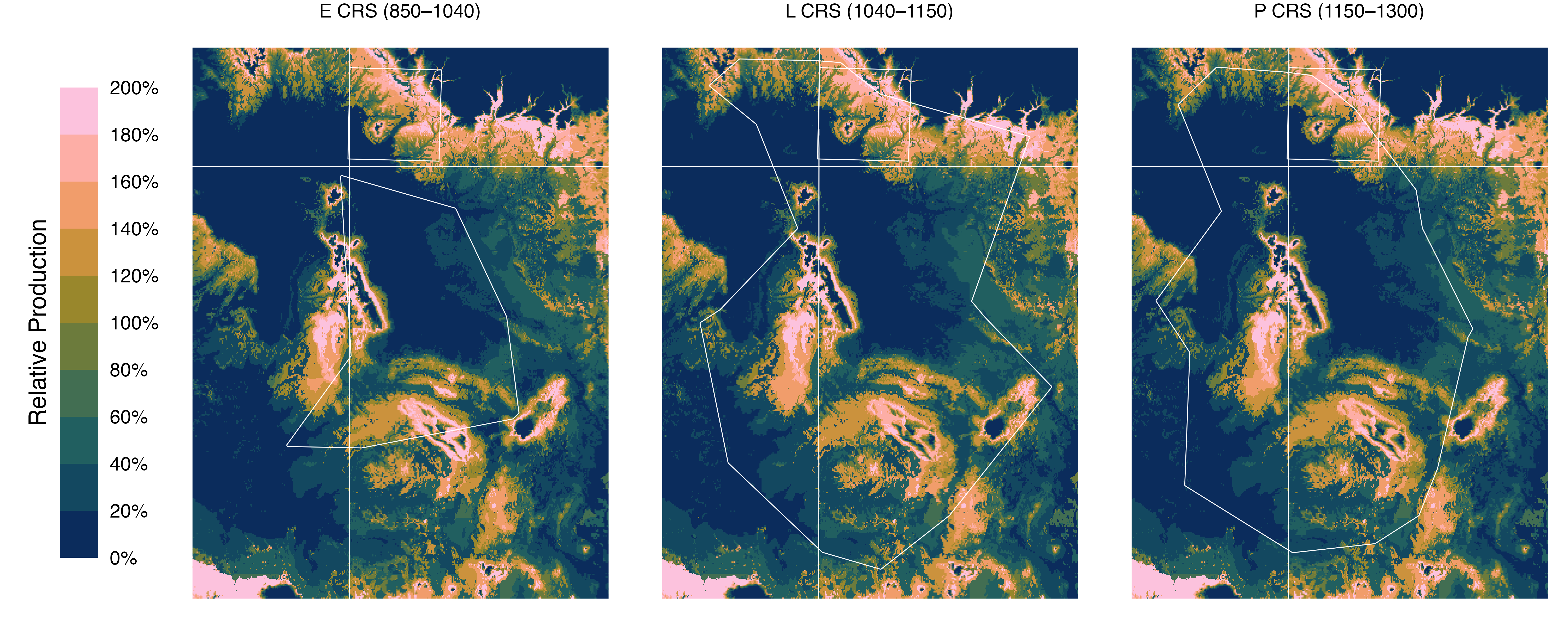
Figure S5: Relative productivity across Chacoan regions during key cultural periods. We scaled niche-attenuated NPP values from each time period relative to the average value in the Central Mesa Verde region (set to 1) to create a unitless measure of agricultural potential. This relative comparison highlights spatial differences in productive capacity across Chacoan regions from A.D. 850 to 1300.
Finally, we bring all of the details together to calculate the statistics and demographic estimates presented in Table 2. See tables/Table_2_250.xlsx for output.
Code
vepiin_area <- chaco_regions %>% dplyr::filter(region =="VEPIIN (850–1300)") %>% sf::st_area() %>% units::set_units("km^2")footnote <-"ᵃas graphed in Schwindt et al. (2016:Figure 3)ᵇcalculated as (Mean proportion potentially productive land, VEPIIN) x ~4,566 sq kmᶜcalculated as (Mean potentially productive sq km, CRS) x (people/potentially productive sq km, VEPIIN) ᵈMomentary Population Estimate, CRS, x Average Productivity Relative to VEPIIN areaᵉterminal date as used by Van Dyke et al. (2016); 1280 used here"crs_niche <- maize_farming_niche %>% dplyr::bind_rows(.id ="region") %>% dplyr::mutate(start =str_extract(region, "\\d+(?=–)"),end =str_extract(region, "(?<=–)\\d+"), dplyr::across(c(start, end), as.integer)) %>% dplyr::filter(between(year, start, end)) %>% dplyr::group_by(start, end, region) %>% dplyr::summarise(`Mean p potentially dry-farmable land, CRS`=mean(mean, na.rm =TRUE),.groups ="drop") %>% dplyr::arrange(region) %>% dplyr::right_join( chaco_regions %>% dplyr::mutate(Area = sf::st_area(geometry) %>% units::set_units("km^2")) %>% sf::st_drop_geometry() ) %>% dplyr::mutate(`Mean potentially dry-farmable sq km, CRS`=`Mean p potentially dry-farmable land, CRS`* Area,region =factor(region, levels =c("E CRS (850–1040)","L CRS (1040–1150)","P CRS (1150–1300)","VEPIIN (850–1300)" ),ordered =TRUE ) )#> Joining with `by = join_by(region)`vepiin_population <- readxl::read_excel("data-raw/Schwindt2016_Table2.xlsx") %>% dplyr::rename(`VEP Start`= Start, `VEP End`= End) %>% tidyr::pivot_longer(!c(`VEP Start`, `VEP End`),names_to ="type",values_to ="Momentary Population Estimate, VEPIINᵃ") %>% tidyr::separate_wider_delim(type, delim =" — ", names =c("subregion", "type")) %>% dplyr::filter(subregion =="Study Area Total", type !="80% CI") %>% dplyr::group_by(`VEP Start`,`VEP End`, subregion) %>% dplyr::summarise(`Momentary Population Estimate, VEPIINᵃ`=sum(`Momentary Population Estimate, VEPIINᵃ`,na.rm =TRUE) ) %>% tidyr::unite("VEP Periods (VEPIIN area ≈ 4,566 sq km)", c(`VEP Start`,`VEP End`),sep =" – ",remove =FALSE) %>% dplyr::select(-subregion) #> `summarise()` has grouped output by 'VEP Start', 'VEP End'. You can override#> using the `.groups` argument.vepiin_population %<>%# dplyr::mutate(dplyr::across(c(`begin (CE)`, `end (CE)`), as.integer)) %>% dplyr::rowwise() %>% dplyr::mutate(year =list(tibble::tibble(year =`VEP Start`:`VEP End`))) %>% tidyr::unnest(year) %>% dplyr::left_join(maize_farming_niche$`VEPIIN (850–1300)`) %>% dplyr::group_by(`VEP Start`, `VEP End`, `VEP Periods (VEPIIN area ≈ 4,566 sq km)`) %>% dplyr::summarise(`Mean p dry-farmable land, VEPIIN`=mean(mean),.groups ="drop") %>% dplyr::arrange(`VEP Start`) %>% dplyr::select(!c(`VEP Start`, `VEP End`)) %>% dplyr::left_join(vepiin_population) %>% dplyr::mutate(`People/dry-farmable sq km, VEPIINᵇ`=`Momentary Population Estimate, VEPIINᵃ`/ (`Mean p dry-farmable land, VEPIIN`* vepiin_area) )#> Joining with `by = join_by(year)`#> Joining with `by = join_by(`VEP Periods (VEPIIN area ≈ 4,566 sq km)`)`vepiin_population_final <- vepiin_population %>% dplyr::mutate(`VEP Periods (VEPIIN area ≈ 4,566 sq km)`,`Mean p dry-farmable land, VEPIIN`=round(`Mean p dry-farmable land, VEPIIN`, 2),`Momentary Population Estimate, VEPIINᵃ`= scales::label_comma()(`Momentary Population Estimate, VEPIINᵃ`),`People/dry-farmable sq km, VEPIINᵇ`=round(units::drop_units(`People/dry-farmable sq km, VEPIINᵇ`), 2),.keep ="none" )crs_population_final <- dplyr::cross_join(crs_niche, vepiin_population) %>% dplyr::filter( dplyr::between(`VEP Start`, start, end) | dplyr::between(`VEP End`, start, end) ) %>% dplyr::group_by( dplyr::across( dplyr::all_of(names(crs_niche) ) ) ) %>% dplyr::summarise(`Mean People/dry-farmable sq km, VEPIINᵇ`=mean(`People/dry-farmable sq km, VEPIINᵇ`) %>% units::drop_units(),`SD People/dry-farmable sq km, VEPIINᵇ`=sd(`People/dry-farmable sq km, VEPIINᵇ`),.groups ="drop" ) %>% dplyr::mutate(`MPE, CRS, meanᶜ`=`Mean potentially dry-farmable sq km, CRS`*`Mean People/dry-farmable sq km, VEPIINᵇ`,`MPE, CRS, lowerᶜ`=`Mean potentially dry-farmable sq km, CRS`* (`Mean People/dry-farmable sq km, VEPIINᵇ`-`SD People/dry-farmable sq km, VEPIINᵇ`),`MPE, CRS, upperᶜ`=`Mean potentially dry-farmable sq km, CRS`* (`Mean People/dry-farmable sq km, VEPIINᵇ`+`SD People/dry-farmable sq km, VEPIINᵇ`) ) %>% dplyr::arrange(region) %>% dplyr::left_join(relative_production_regions) %>% dplyr::rename(`Average Productivity Relative to VEPIIN area`= relative_productivity) %>% dplyr::mutate(`CMPE, CRS, meanᵈ`=`MPE, CRS, meanᶜ`*`Average Productivity Relative to VEPIIN area`,`CMPE, CRS, lowerᵈ`=`MPE, CRS, lowerᶜ`*`Average Productivity Relative to VEPIIN area`,`CMPE, CRS, upperᵈ`=`MPE, CRS, upperᶜ`*`Average Productivity Relative to VEPIIN area`,`Momentary Population Estimate, CRS, mean (range)ᶜ`=paste0( scales::label_comma()(units::drop_units(`MPE, CRS, meanᶜ`))," (", scales::label_comma()(units::drop_units(`MPE, CRS, lowerᶜ`))," – ", scales::label_comma()(units::drop_units(`MPE, CRS, upperᶜ`)),")" ),`Corrected Momentary Population Estimate, CRS, mean (range)ᵈ`=paste0( scales::label_comma()(units::drop_units(`CMPE, CRS, meanᵈ`))," (", scales::label_comma()(units::drop_units(`CMPE, CRS, lowerᵈ`))," – ", scales::label_comma()(units::drop_units(`CMPE, CRS, upperᵈ`)),")" ),`CRS Periods, dates, size`=paste0( region,", ", scales::label_comma()(units::drop_units(Area))," sq km" ),`People/dry-farmable sq km, VEPIIN (mean ± SD)ᵇ`=paste0(round(`Mean People/dry-farmable sq km, VEPIINᵇ`, 2)," ± ",round(`SD People/dry-farmable sq km, VEPIINᵇ`, 2) ),`Mean potentially dry-farmable sq km, CRS`= scales::label_comma()(units::drop_units(`Mean potentially dry-farmable sq km, CRS`)) ) %>% dplyr::mutate(`CRS Periods, dates, size`, `People/dry-farmable sq km, VEPIIN (mean ± SD)ᵇ`,`Mean p potentially dry-farmable land, CRS`=round(`Mean p potentially dry-farmable land, CRS`, 3),`Mean potentially dry-farmable sq km, CRS`,`Momentary Population Estimate, CRS, mean (range)ᶜ`,`Average Productivity Relative to VEPIIN area`=round(`Average Productivity Relative to VEPIIN area`, 2),`Corrected Momentary Population Estimate, CRS, mean (range)ᵈ`,.keep ="none" ) %>% dplyr::select(`CRS Periods, dates, size`, `People/dry-farmable sq km, VEPIIN (mean ± SD)ᵇ`,`Mean p potentially dry-farmable land, CRS`,`Mean potentially dry-farmable sq km, CRS`,`Momentary Population Estimate, CRS, mean (range)ᶜ`,`Average Productivity Relative to VEPIIN area`,`Corrected Momentary Population Estimate, CRS, mean (range)ᵈ`)#> Joining with `by = join_by(region)`list(`VEPIIN`= vepiin_population_final,`Chaco Regional System`= crs_population_final) %>% openxlsx::write.xlsx(file =paste0("tables/Table_2_", ppt_threshold, ".xlsx"),asTable =TRUE,colWidths ="auto" )